• apache-spark
• bucketing
• partition

Partitioning and bucketing are used to improve the reading of data by reducing the cost of shuffles, the need for serialization, and the amount of network traffic.

Partitioning in Spark

Apache Spark’s speed in processing huge amounts of data is one of its primary selling points. Spark’s speed comes from its ability to allow developers to run multiple tasks in parallel and independently across hundreds of machines in a cluster or across multiple cores on a desktop. It’s all possible because Apache Spark RDDs serve as the main interface. These RDDs are partitioned and run in parallel behind the scenes.

So, what exactly is the partition in Spark? Spark organizes data into smaller pieces called “partitions”, each of which is kept on a separate node in the cluster. Each partition is an atomic chunk of data. We can think of partition as a subset of our data. Simply said, it’s a subset of the superset.

Parallelism

Partitions are the fundamental building blocks of parallelism in Apache Spark. Spark’s parallelism enables developers to parallelly execute several tasks across a large number of nodes in a cluster.

Co-location

Partitioning can also deliver a significant speed benefit by reducing the amount of data to be shuffled across the network. If RDDs are too large to fit on a single node, they must be partitioned (distributed) across many nodes. Apache Spark automatically partitions RDDs and distributes them across different nodes.

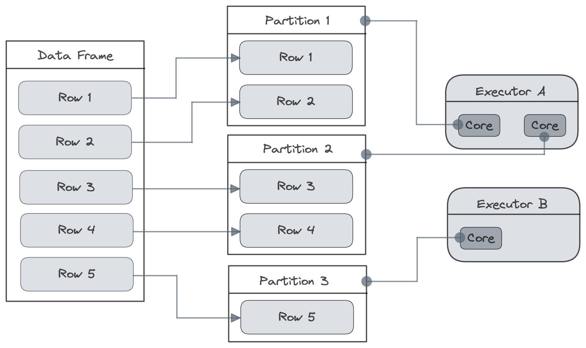
Figure 1: Data Partitioned by Spark.

Spark is a distributed computing system, so it can operate on data partitons in parallel. A transformation or any sort of computation on a data partitons is called a task and each task generally takes place on one core. As there is one task for every partition, the total number of tasks is the same as the total number of partitions. Optimal partitioning in Spark strikes a balance between read performance and write performance.

Please take the following considerations into account:

• Too many partitions: Too many partitions can slow down the time it takes to read and force Spark to create more tasks to process the data, which could cause the driver to get an “out of memory” error.
• Too many small partitions could waste a lot of time because the cluster would spend more time coordinating tasks and sending data between workers than actually doing the job.
• Overly large partitions can even cause executor “out of memory” errors.
• Using a small number of large partitions may leave some worker cores idle. If one of the workers is falling behind the other, we may have to wait a long time for the last task to be completed. If a worker goes down, we’ll have to reprocess a huge amount of data.
• Few or lack of partitions: On the other hand, a lack of or few partitions may indicate that Spark’s parallelism is not being fully utilized, resulting in long computation and write times. Furthermore, having few partitions may result in skewed data and inefficient resource use.
• Data skewness: We refer to data as “skewed” when it is not evenly distributed among workers. In Apache Spark, transformations like join, groupBy, and orderBy change data partitioning, which results in data skewness. Common effects of skewed data include the following:
  • Slow running stages or tasks: Certain operations will take very long to complete because of the huge volume of data that a particular worker must process.
  • Spilling data to disk: In the event that more data is not able to fit in the memory of a worker, it must be written to disk.
  • Out-of-memory error: If worker runs out of disk space, an error is thrown.

Spark generally does a good job splitting data into partitons to ensure parallelism and efficient computing. However, when dealing with very large data sets, it is sometimes necessary to manually adjust partitions to ensure optimal performance. As a rule of thumb, 128 megabytes is a good size for a data partition when dealing with data sets above 1 gigabyte. That is, # Partitions = Dataset Size (mb) / 128 mb.

To get us started with partitioning, here are some fundamentals:

• Every node (worker) in a Spark cluster contains one or more partitions of any size.
• By default, Spark tries to set the number of partitions automatically based on the total number of cores on all the executor nodes. This is the most effective method for determining the total number of spark partitions in an RDD. However, we can manually set it by passing it as a second parameter to parallelize (for example, sc.parallelize(data, 10)). 
• The number of partitions in Spark is configurable.
• Only one partition is processed by one executor at a time, so the size and number of partitions handed to the executor are directly proportional to the time it takes to complete them.

Types of partitioning

We bring in the data, transform it, and then either write it somewhere else or display it on our console or screen. This allows us to further divide Spark partitions into three categories. 

• Input partition - Control the size of the partition using spark.sql.files.maxPartitionBytes
• Output partition - Control the size of the partition using coalesce (to reduce partition) and repartition (to reduce or increase partition)
• Shuffle partition - Control the partition count using spark.sql.shuffle.partitions

Input partition

When a job is submitted for processing, each data partition is sent to the specific executors. Each executor processes one partition at a time. Hence, the time it takes each executor to process data is directly proportional to the size and number of partitions. The more partitions there are, the more work will be distributed (shuffled) among the executors. There will also be fewer partitions. This means that processing will be done faster and in larger chunks.

What influences the input partition?

Since the input partition is a critical parameter for performance, how should we control the size of the partition? Spark has a property called spark.sql.files.maxPartitionBytes that can be used to control the number of bytes that are packed into a single partition when reading files, and if we want to check the number of partitions, we can do it by using the method rdd.getNumPartitions(). The another alternative method to get the number of partitions is rdd.partitions.size().

Note: The default value for spark.sql.files.maxPartitionBytes property is 134217728 (128 MB). In the event that the size of either the input file block or a single partition is more than 128 MB, Spark will split the read into multiple partitions. This configuration is effective only when using file-based sources such as Parquet, JSON and ORC.

By using the aforementioned property and method, we can know the default number of partitions being created and then modify it to our liking. We want to control the size of the partitions because we don’t want too much data shuffled around. Because each partition is sent to an executor, the number of partitions determines how much data is shuffled around.

Output partition

Output partition is essential whenever we are reading data for further processing. If there are several partitions, data will be spread over many files, making it more time-consuming to search for specific criteria in the first query. Whenever our job is finished and we are writing back the data, at that point, the output partition determines the number of files that will get returned to our disk. The larger the number of partitions, the larger the number of files. The total number of files generated is directly proportional to the number of output partitions.

Also, our memory utilization will be higher while processing the metadata table, as it contains several partitions. Having said that, the output partition influences how we write the data back into the disk after the job is completed.

What influences the output partition?

There are two methods that can influence the way our data is written:

• repartition - The repartitioning operation reduces or increases the number of partitions. This is a costly operation that involves shuffling all the data over the network and redistributing it so that it is spread out evenly. Data is serialized, transferred, and then de-serialized throughout this process.
• coalesce - The coalesce operation uses existing partitions and reduces (doesn’t increase) the number of partitions to minimize the amount of data that’s shuffled. Coalesce results in partitions that contain different amounts of data. In most cases, the coalesce runs faster than the repartition operation.

By using coalesce and repartition, we can limit the output to a certain number of files or tasks.

Shuffle partition

In cases of wide transformations, where data is required from other partitions, Spark performs a data shuffle. We can’t avoid making such wide transformations, but we can reduce the impact on performance by configuring parameters. Wide transformations use shuffle partitions to shuffle data. We can control the shuffle partition using spark.sql.shuffle.partitions.

Note: The number of partitions is fixed at 200 regardless of the data’s size or the number of executors.

How to set shuffle partition?

When the data is small, the number of partitions should be reduced; otherwise, too many partitions containing less data will be created, resulting in too many tasks with less data to process.

When working with a big dataset, it may be beneficial to increase the shuffle partition from the default value of 200.

Spark partitioning strategies

Apache Spark supports two types of partitioning strategies:

• Hash partitioning (Default)
• Range partitioning

Let’s understand the rationale for the need for a variety of partitioning strategies. A suitable data partitioning strategy will enable us to reduce the skew in the data. Keep in mind that Spark limits the size of a partition to 2 GB, although there may be cases when a single key includes several relevant records that add up to more than 2 GB in total. If we have partitioned our data on that specific key, then we are going to have problems shuffling that data; we will get errors. So, picking the right partitioning strategy is very important. It also helps us get the best performance out of different operations like join and groupby.

Choosing the right partitioning strategy will help us to co-locate the data. The term “collate the data” refers to the fact that data that is processed together is also stored together. By doing so, we may avoid redistributing data around the cluster every time we do a groupby or join operation.

Partitioning decisions are influenced by a wide variety of factors, including:

• Available resources (CPU, memory, and network)
• Transformation used to derive RDD -

How do we get the right partitions?

Recommended number of partitions

Apache Spark can only run a single concurrent task for every partition of an RDD, up to the number of available cores in our cluster (and probably 2 to 3 times that). Hence, it is common practice to choose a good number of partitions equal to or more than the number of executors to maximize parallelism. For example, if we have eight worker nodes and each node has four CPU cores, we may set the number of partitions to be anywhere from 64 (2 x 8 x 4) to 96 (3 x 8 x 4).

By calling sc.defaultParallelism we can get the default level of parallelism defined on SparkContext. The maximum size of a partition is limited by how much memory an executor has.

Recommended partition size

The average partition size ranges from 100 MB to 1000 MB. For instance, if we have 30 GB of data to be processed, there should be anywhere between 30 (30 gb / 1000 mb) and 300 (30 gb / 100 mb) partitions.

Other factors to be considered

It is important to understand and carefully choose the right operators for actions like reduceByKey or aggregateByKey so that our driver is not put under pressure and the tasks are properly executed on executors. 

When data is skewed, it is recommended to use an appropriate key that can spread the load evenly. Sometimes, it may not be clear which re-partitioning key should be used to make sure data is evenly distributed. In these situations, we can use methods like salting, which involves adding a new fake or random key and using it along with the current key for better distribution of data. This is how it works: saltKey = actualJoinKey + randomFakeKey.

Hive partition vs. Spark partition

Hive partition is not the same as Spark partition. The two are completely different. They are both subsets of the superset, but a Spark partition is a piece of data that has been broken down so that it can be processed in parallel in memory. Hive partition is in disk storage and persistence.

---

Bucketing in Spark

Bucketing is an optimisation feature that Apache Spark (also in Apache Hive) has supported since version 2.0. It’s a way to improve performance by dividing data into smaller, manageable portions called “buckets” to identify data partitioning as it’s being written down. This feature is intended to improve the efficiency of reading same data. This efficiency improvement is mostly about getting rid of shuffles (also called exchanges) in join and aggregation queries.

Apache Hive popularised buckets, and Apache Spark added their support.

Shuffle is a very expensive operation as it moves the data between executors or even across worker nodes in a cluster. Hence, it should be avoided wherever feasible. When there is a problem with the performance of Spark jobs, we should examine the transformations that involve shuffling.

With bucketing, we can pre-shuffle and store the data in a pre-shuffled form. It controls the physical arrangement of the data, thus we shuffle the data beforehand to prevent having to do it later on.

Sorting the bucket

In addition to bucketing, we can also do sorting, which sorts each bucket according to the given fields. However, the opposite is not possible; we cannot sort without bucketing.

Configure bucketing

Note that bucketing is enabled by default. Spark controls whether or not it should be enabled using the configuration property spark.sql.sources.bucketing.enabled.

How to create buckets?

In Spark API, the bucketBy method can be used for this purpose.

bucketBy(n, field1, field2, ...)

The first argument specifies the number of buckets to generate. The number of buckets is equal to the number of files generated.

# In Python
df.write\
    .bucketBy(16, "key")\
    .sortBy("value")\
    .saveAsTable("table_name")

Bucketing applicable only to persistent tables

Only persistent tables can be used for bucketing and sorting. We can only use the saveAsTable method; we can’t use the save method.